Solving a problem with ADMM

We will briefly explain the ADMM component and go through an example. Note that the current capabilities of this class are limited, more features are coming soon (tm).

ADMM in elsa

Alternating Direction Method of Multipliers is an algorithm which provides the grounds for solving a certain class of problems. It combines the superior convergence properties of the method of multipliers along with the decomposability of the dual ascent algorithm [1].

ADMM solves problems of the form

minimize $f(x) + g(z)$

subject to $Ax + Bz = c$.

A Least Absolute Shrinkage and Selection Operator problem is of the form,

minimize $\frac{1}{2}\|Ax - b\|^{2}_{2} + \lambda \|x\|_{1}$

elsa offers the LASSOProblem class to encapsulate such problems. Using variable splitting, this can be rewritten to

minimize $\frac{1}{2}\|Ax - b\|^{2}_{2} + \lambda \|z\|_{1}$

subject to $x - z = 0$.

Now we have a SplittingProblem. We observe that this pattern abides by the form of problems that ADMM can solve, in which $f(x) = \frac{1}{2}\|Ax - b\|^{2}_{2}$$ and $g(z)=lambda |z|_{1}, where $A$ is the identity matrix, $B$ is $-1$ times the identity matrix, and $c$ is the vector $0$. The objects of this class can be built by providing a Functional f and a RegularizationTerm g(or a vector of them), so we use the aforementioned $f$ and $g$.

ADMM then solves that problem by alternating updates of its variables. We’re showing here the scaled form which we also use.

\[x_{k+1} = argmin_{x}(f(x) + \frac{\rho}{2} \|Ax + Bz_{k} - c + u_{k}\|^{2}_{2})\]

\[z_{k+1} = argmin_{z}(g(z) + \frac{\rho}{2} \|Ax_{k+1} + Bz - c + u_{k}\|^{2}_{2})\]

\[u_{k+1} = u_{k} + Ax_{k+1} + Bz_{k+1} - c\]

The selection of the regularization parameter lambda, which is introduced in the next section, and the coupling parameter rho, is not quite straightforward. In this instance, we’ve chosen to set the value of rho to 1, and the value of lambda to 1/2. It is evident that the result of ADMM depends on both of these. More information on this, is provided by Wieczorek et al. [2].

Solving a toy inverse problem using ADMM

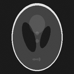
We start by generating a modified 2D Shepp-Logan phantom by calling

IndexVector_t size(2);
size << 256, 256;
auto phantom = phantoms::modifiedSheppLogan<real_t>(size);

This generates the following image,

We generate a circular acquisition trajectory using CircleTrajectoryGenerator,

index_t numAngles{180}, arc{360};
auto distance = static_cast<real_t>(size(0));
auto sinoDescriptor = CircleTrajectoryGenerator::createTrajectory(numAngles, phantom.getDataDescriptor(), arc,
                                                                  distance * 100.0f, distance);

We continue by creating a projector of type SiddonsMethod, which utilizes the sinoDescriptor data descriptor above.

SiddonsMethod projector(dynamic_cast<const VolumeDescriptor&>(phantom.getDataDescriptor()), *sinoDescriptor);

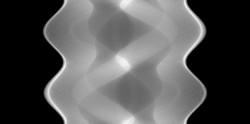
Simulate the sinogram and write it to an EDF file,

auto sinogram = projector.apply(phantom);

EDF::write(sinogram, "2dsinogram.edf");

This generates the following sinogram,

ADMM requires a SplittingProblem to solve. As mentioned above, we will utilize a LASSOProblem object to construct that, which requires setting up the weighted least squares problem and the `L1 regularizer <https://en.wikipedia.org/wiki/Regularization_\(mathematics\>`_). We do that as follows,

WLSProblem wlsProblem(projector, sinogram);

real_t lambda = 0.5f;
L1Norm regFunc(projector.getDomainDescriptor());
RegularizationTerm regTerm(lambda, regFunc);

We continue by creating the $Ax + Bz = c$ constraint, which in our scenario is simply $x - z = 0$,

const DataDescriptor& regDatDescriptor = regTerm.getFunctional().getDomainDescriptor();

Identity idOp(regDatDescriptor); // A
Scaling<real_t> negativeIdOp(regDatDescriptor, -1); // B
DataContainer dZero(regDatDescriptor); // c
dZero = 0; // 0

Constraint constraint(idOp, negativeIdOp, dZero);

Now let’s create the SplittingProblem object which utilizes the two parts and the constraint

SplittingProblem splittingProblem(wlsProblem.getDataTerm(), regTerm, constraint);

Finally, we build the ADMM solver. We can specify the solvers as template parameters. Note that as of currently, we support subclasses of Solver and ProximityOperator for the first and second template respectively. We chose to specify the conjugate gradient solver as CGLS along with the shrinkage/soft-thresholding operator as ProximalL1

ADMM<CGLS, ProximalL1> admm(splittingProblem);

We can now reconstruct the phantom! We do this simply by

index_t noIterations{10};
auto admmReconstruction = admm.solve(noIterations);

Writing the output in an EDF file makes the visualization easier.

EDF::write(admmReconstruction, "2dreconstruction_admm.edf");

After 10 iterations of ADMM, the phantom reconstruction is generated. From here we can do a side-by-side comparison of the original phantom and its reconstruction,

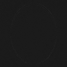
Finally, we can also create the element-wise difference image between the two by simply writing,

DataContainer phantom = EDF::read("2dphantom.edf");
DataContainer phantomRecon = EDF::read("2dreconstruction_admm.edf");

DataContainer diffImage = phantom - phantomRecon;

EDF::write(diffImage, "2ddifference_image.edf");

which displays the following image

References

[1] S. Boyd, N. Parikh, E. Chu, B. Peleato and J. Eckstein. Distributed Optimization and Statistical Learning via the Alternating Direction Method of Multipliers. Foundations and Trends in Machine Learning 3(1), 2011. DOI: 10.1561/2200000016

[2] M. Wieczorek, J. Frikel, J. Vogel, E. Eggl, F. Kopp, P.B. Noel, F. Pfeiffer, L. Demart, T. Lasser. X-ray computed tomography using curvelet sparse regularization. Medical Physics 42(4), 2015. DOI: 10.1118/1.4914368