Getting started

Table of Contents

• Getting started

  • A first example

  • Sequential Networks

  • Graphs and pretty printing

  • Compiling a model

  • Train a model

A first example

Let’s start with a first example and build a network to learn the famous MNIST task which consists of 60.000 images of handwritten digits with height and width both 28.

We start by defining a VolumeDescriptor describing the input shape of a single MNIST image and then define our first network layer.

VolumeDescriptor inputDescriptor{{28, 28, 1}};

auto input = ml::Input(inputDescriptor, /* batch-size */ 10);

In this first example we design a fully-connected network. We must therefore flatten our input using a Flatten layer. We set the input of flatten to be our input layer defined above;

auto flatten = ml::Flatten();
flatten.setInput(&input);

Let’s add a Dense layer and set the input. The Dense layer is defined by specifying the number of neurons (128 in this case) and the activation function. Again, we set the input of dense to be flatten.

// A dense layer with 128 neurons and Relu activation
auto dense = ml::Dense(128, ml::Activation::Relu);
dense.setInput(&flatten);

Finally we add a second Dense layer, followed by a Softmax layer:

// A dense layer with 10 neurons and Relu activation
auto dense2 = ml::Dense(10, ml::Activation::Relu);
dense2.setInput(&dense);

auto softmax = ml::Softmax();
softmax.setInput(&dense2);

Now it’s time to construct a Model out of the layers above which works just by specifying the input and output of our network

auto model = ml::Model(&input, &softmax);

Sequential Networks

Since our fully-connected network above consists of layers with at most one input and at most one output we call such a network sequential, again following Keras’s naming convention.

In the case of a sequential network we have an easier way to build out model. The above network can also be constructed by the following snippet:

auto model = ml::Sequential(ml::Input(inputDesc, /* batch-size */ 1),
                            ml::Dense(128, ml::Activation::Relu),
                            ml::Dense(10, ml::Activation::Relu),
                            ml::Softmax());

Graphs and pretty printing

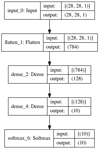
While constructing a model, elsa defines an internal graph representation of the network. Observing this graph can be helpful. Elsa exports network graphs in Graphviz’ DOT language:

ml::Utils::Plotting::modelToDot(model, "myModel.dot");

By using e.g.

$ dot -Tpng myModel.dot > myModel.png

the network model defined in the previous section is plotted as

Another possibility to observe the architecture of a model is to just print the model to console:

std::cout << model << "\n";

In our example this would result in

Model:
________________________________________________________________________________
Layer (type)                       Output Shape        Param #   Connected to
================================================================================
input_0 (Input)                    (28,  28,   1)      0         flatten_1
________________________________________________________________________________
flatten_1 (Flatten)                (784)               0         dense_2
________________________________________________________________________________
dense_2 (Dense)                    (128)               100480    dense_4
________________________________________________________________________________
dense_4 (Dense)                    (10)                1290      softmax_6
________________________________________________________________________________
softmax_6 (Softmax)                (10)                0
================================================================================
Total trainable params: 101770
________________________________________________________________________________

Compiling a model

So far we only defined what we call a front-end model. To really do something meaningful we need to compile the model. This is also the point where we set the loss function we want to use as well as the optimizer.

While compiling a model elsa performs a lot of detail work under the hood. In particular backend resources get allocated.

Let’s compile our toy MNIST model with a SparseCategoricalCrossentropy loss and the well known Adam optimizer:

// Define an Adam optimizer
auto opt = ml::Adam();

// Compile the model
model.compile(ml::SparseCategoricalCrossentropy(), &opt);

After the model is compile we are ready for training or inference.

Train a model

Training a model is straight forward and most of the work will be preparing training data which is of course independant of elsa. Assume we bundled our MNIST images into a std::vector<DataContainer> inputs and our labels into labels respectively.

Following Keras we can traing our model as easy as

model.fit(inputs, labels, /* epochs */ 10);